Introduction#
At its core, euv_fitting is about providing tools to automate the analysis of EUV spectra. This document serves as a guide for understanding how NIST spectra are represented and how this module processes them.
Spectra Contents#
The CCD Camera that produces NIST spectra stores them as binary .SPE files. The data in these files is typically a (N x 2048) array, where N is the number of frames. Each frame represents a minute of data collection, so a (10 x 2048) array represents a spectra that was taken over ten minutes. The 2048 columns correspond to the 2048 pixels on the CCD camera. Pixels (or channels) are 0-indexed, so the last channel number is 2047. As channel number increases, so does wavelength. Finding the relationship between channel number and wavelength is not trivial and is the main focus of the euv_fitting package.
In addition to the intensity data present in each .SPE file, metadata about the time,
date, and CCD camera parameters when the spectra was taken are also included.
The SpeReader converts the binary data
stored in a .SPE file into NumPy arrays and a metadata dictionary, as in the example below.
from euv_fitting.calibrate.utils import SpeReader

S = SpeReader('../euv_fitting/calibrate/270.spe')
img = S.load_img()

print(f'Spectra has shape {img.shape}')
print('With metadata:')
S.print_metadata()
Spectra has shape (5, 2048)
With metadata:
gain: 3
adcrate: 6
adcresolution: 9
temp: 0.0
rawdate: 09Jan2020
rawtime: 114204
comments: ('', '', '', '', '')
We can plot this spectra to get an idea of its composition.
import matplotlib.pyplot as plt

plt.plot(img.T)
plt.xlabel('Channel Number [-]')
plt.ylabel('Intensity [ADU]')
plt.title('Neon Spectra')

plt.legend([f'Frame {i + 1}' for i in range(img.shape[0])])
plt.show()
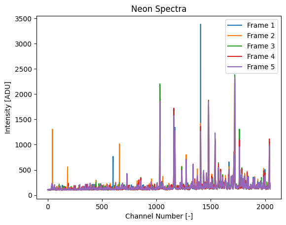
Each color in the original plot represents a different frame in the spectra. One thing to notice are that some frames have high intensity at channels that have a much lower intensity than other frames. These single-frame spikes come from cosmic rays, and do not provide any useful experimental information.
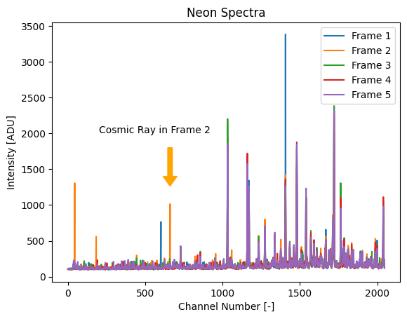
To remove these, we can use a CosmicRayFilter
on our spectra. This has the added effect of collapsing the five frames into one
spectra, resulting in higher intensity values.
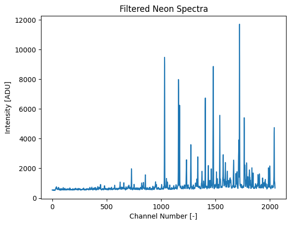
from euv_fitting.calibrate.utils import CosmicRayFilter

CRF = CosmicRayFilter()
img_filtered = CRF.apply(img)

plt.plot(img_filtered)
plt.xlabel('Channel Number [-]')
plt.ylabel('Intensity [ADU]')
plt.title('Filtered Neon Spectra')
plt.show()
Sample Calibration#
Now that we have removed the cosmic rays from our spectra, we can create our calibration. A calibration is defined by a third order polynomial, or
where \(x\) is the channel number, \(\lambda\) is the wavelength at that channel number, and \(k_i\) is the ith calibration coefficient. Finding the calibration amounts to determining the values and uncertainties of each calibration coefficient.
Currently, support is included for calibrations based on Neon, Background, and Argon spectra.
To calibrate this neon spectra, we first create a Distance_Calibrator
object, specifying the number of peaks to fit and the element of the spectra.
from euv_fitting.calibrate.calibrators import Distance_Calibrator

Ne_Cal = Distance_Calibrator(img_filtered, 'Ne', num_peaks = 25)
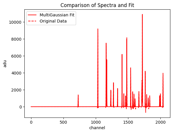
To verify that the fit completed successfully, we can plot the original data and the predicted values on the same axis. Information about all fit peaks is stored in Ne_Cal.multi.gauss_data, which is an (N x 3 x 2) array, where N is the number of peaks. Each row represents the [[amplitude, amplitude_std], [center, center_std], [sigma, sigma_std]] of a different peak.
Ne_Cal.multi.plot_fit()
print('Printing information for the 6th peak fit.')
print(Ne_Cal.multi.gauss_data[5, :, :])
Printing information for the 6th peak fit.
[[1.40659451e+03 2.75744772e-02]
 [1.67844924e+04 4.89162106e+02]
 [1.08213360e+00 3.04436770e-02]]
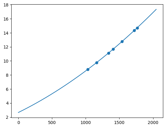
To finish the calibration, we first call the Ne_Cal.calibrate() method, which identifies well known calibration lines in the spectra. Next, we call Ne_Cal.fit() which uses the identified calibration lines to calculate the calibration coefficients.
Ne_Cal.calibrate()
Ne_Cal.fit()
Ne_Cal.plot()
Ne_Cal.print_info()
selecting best peaks
K0 = 2.658095554982152±0.05891793355062553
K1 = 0.004718422685678915±0.00013338296308877779
K2 = 1.2039248254098424e-06±9.865691255385293e-08
K3 = -2.7454680289512726e-12±2.386810238057546e-11
Highest/Average channel uncertainty 4.93e-04 / 2.63e-04
Highest/Average wavelength uncertainty 1.80e-03 / 7.06e-04
Systematic Uncertainty: 0
Unadjusted Chi-square: 0.9989862473518202
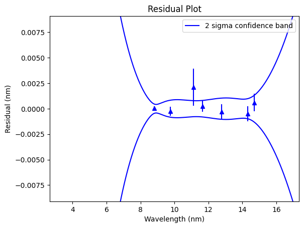
The calibration coefficients are accessible through the Ne_Cal.popt attribute. We can also plot the residuals of our fit and the literature wavelength of the calibration lines:
Ne_Cal.residual_plot()