Uncertainties#

No calibration is complete without a thorough understanding of the uncertainty in your results and where that uncertainty comes from. This section is a review of the types of the uncertainty present in calibrations, how to access them, and common mistakes made when calculating uncertainties.

Types of Uncertainty#

Channel Uncertainty (Centroid Uncertainty)#

Channel uncertainty comes from the inherent statistical uncertainty in the peak fitting process. A peak with a center at channel 1000 looks almost identical to a peak with a center at channel 1000.1, especially if you only saw a few photons from that peak. A channel uncertainty can be converted to a wavelength uncertainty using the function

\[u_{x,nm} = f_{cal}'(x) * u_{x,ch}\]

Where \(u_{x,nm}\) is the uncertainty from peak fitting in nm, \(u_{x,ch}\) is the uncertainty in channels, \(f_{cal}(x)'\) is the derivative of the calibration function evaluated at x.

As an example, consider you know the calibration function is:

\[f_{cal}(x) = 4 nm + 1 * 10^{-6} \frac{nm}{{ch}^2} x ^ 2\]

Which has the derivative

\[f_{cal}(x) = 2 * {10^{-6}} \frac{nm}{{ch}^2} x\]

A line at channel 500 with a channel uncertainty of +/- 1 nm would have an effective wavelength uncertainty of:

\[ \begin{align}\begin{aligned}u_{x,nm} = 2 * {10^ {-6}} \frac{nm}{{ch}^2} 500 ch * 1 ch\\u_{x,nm} = 0.001 nm.\end{aligned}\end{align} \]

Literature Wavelength Uncertainty#

The calibration lines are not known exactly, and come with uncertainty values attached as well. We do not have to calculate these, as they are given in other publications.

Systematic Uncertainty#

The calibration drifts over time due to thermal expansion of the grating, small movements of the CCD camera, and other factors. Systematic uncertainty attempts to capture the errors in calibrations that do come from statistical sources. For more information of how systematic uncertainty is estimated, see the section on Estimation of Systematic Uncertainty

Calibration Uncertainty#

Once a calibration has been completed, a scientist needs to know not only what the wavelength is at a certain point, but also how confident they can be in that wavelength. The calibration uncertainty represents the +/- at a predicted wavelength, and changes as channel number changes. In areas where you have many calibration lines, the calibration uncertainty is generally smaller. If there are no close calibration lines, you can expect higher calibration uncertainties.

To obtain the 1 sigma (close to 68% confidence band) calibration uncertainties, use the confidence_bands() method after fitting has been completed.

cb = calibrator.confidence_bands(n_sigma = 1)

#or

cb = calibrator.confidence_bands(n_sigma = 1)
cb = calibrator.cb

cb.shape == (2048,)

cb will be an array of the calibration uncertainty at each channel.

Examples and Best Practices#

One common task for users of euv_fitting is creating a calibration, applying it to another spectra, and then extracting the wavelength and wavelength uncertainty of peaks in that spectra. This example is a template for completing that process and mentions some mistakes to avoid along the way.

First, create a calibration from a Neon and Background file. For more information, see the Calibration Process section.

from euv_fitting.calibrate.utils import SpeReader, CosmicRayFilter
from euv_fitting.calibrate.calibrators import Distance_Calibrator

CRF = CosmicRayFilter()

Ne_spe = SpeReader('./example_data/Example_Neon.SPE')
Bkg_spe = SpeReader('./example_data/Example_Background.SPE')

Ne_img = CRF.apply(Ne_spe.load_img())
Bkg_img = CRF.apply(Bkg_spe.load_img())

Ne_cal = Distance_Calibrator(Ne_img, 'Ne', num_peaks = 25) #specify element and #peaks
Bkg_cal = Distance_Calibrator(Bkg_img, 'Ba', num_peaks = 25) #specify element and #peaks

Ne_cal.calibrate()
Bkg_cal.calibrate()

Ne_cal.join([Bkg_cal])

print('Total Solution Array')
print(Ne_cal.solution_arr)

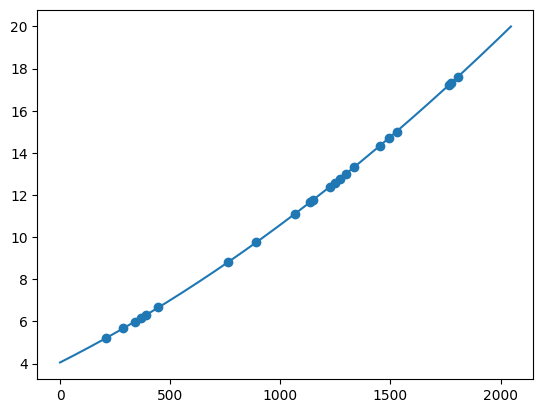
Ne_cal.fit()
Ne_cal.plot()
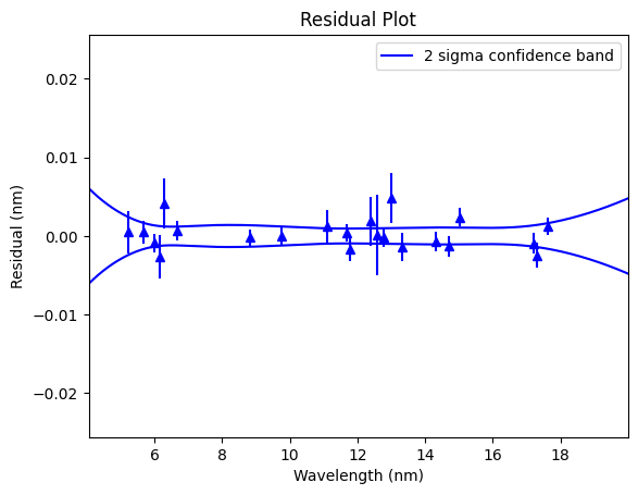
Ne_cal.residual_plot()
Ne_cal.print_info()

selecting best peaks

selecting best peaks

Total Solution Array
[[8.80929000e+00 1.40000000e-04 7.62421231e+02 2.58781802e-02]
 [9.75020000e+00 4.00000000e-04 8.90567351e+02 3.55102613e-02]
 [1.11136000e+01 1.80000000e-03 1.06748262e+03 3.36749072e-02]
 [1.16691000e+01 5.00000000e-04 1.13674959e+03 2.73318275e-02]
 [1.27676000e+01 7.00000000e-04 1.26986371e+03 1.56628562e-02]
 [1.43314000e+01 7.00000000e-04 1.45125753e+03 2.30675110e-02]
 [1.47138000e+01 7.00000000e-04 1.49425996e+03 4.19253220e-02]
 [1.76186000e+01 2.80000000e-04 1.80726417e+03 2.92112055e-02]
 [1.95004000e+01 8.00000000e-04 1.99888699e+03 2.73615248e-02]
 [5.21540000e+00 2.50000000e-03 2.09996430e+02 6.03119420e-02]
 [5.67700000e+00 1.00000000e-03 2.88094113e+02 4.50670806e-02]
 [5.98460000e+00 2.00000000e-04 3.38510633e+02 7.24005140e-02]
 [6.16220000e+00 2.50000000e-03 3.67006855e+02 9.25922924e-02]
 [6.28800000e+00 3.00000000e-03 3.88270099e+02 5.29248232e-02]
 [6.66230000e+00 7.00000000e-04 4.46800576e+02 3.19296907e-02]
 [1.17686000e+01 1.00000000e-03 1.14876942e+03 3.39887742e-02]
 [1.23920000e+01 3.00000000e-03 1.22513586e+03 2.31265415e-02]
 [1.25818000e+01 5.00000000e-03 1.24772767e+03 4.11585546e-02]
 [1.29930000e+01 3.00000000e-03 1.29716876e+03 3.89691709e-02]
 [1.33246000e+01 1.40000000e-03 1.33537973e+03 5.23796173e-02]
 [1.50101000e+01 5.00000000e-04 1.52770709e+03 3.52752553e-02]
 [1.72169000e+01 3.00000000e-04 1.76518033e+03 8.77637881e-02]
 [1.73081000e+01 5.00000000e-04 1.77455803e+03 1.19250428e-01]]

K0 = 4.051760979290335±0.003037473135061028
K1 = 0.005274290727274932±1.1718352123140706e-05
K2 = 1.2887169025469727e-06±1.2352525685988656e-08
K3 = -2.9330230066183045e-11±3.842164006338311e-12
Highest/Average channel uncertainty 1.14e-03 / 3.63e-04
Highest/Average wavelength uncertainty 5.00e-03 / 1.36e-03
Systematic Uncertainty: 0.0010382812499999975
Unadjusted Chi-square: 2.41881744438093

Immediately, we can identify the:

channel uncertainty (fourth column of the solution array)
literature wavelength uncertainty (second column of the solution array)
systemtatic uncertainty (given in the print out)

from euv_fitting.calibrate.utils import MultiBatchGaussian

import numpy as np
import matplotlib.pyplot as plt

#apply the calibration function to our channels to get wavelengths
channels = np.linspace(0, 2047, 2048)
wavelengths = Ne_cal.f3(channels, *Ne_cal.popt)


Ir_spe = SpeReader('./example_data/Example_Neon.SPE')
Ir_img = CRF.apply(Ir_spe.load_img())

#create multibatchgaussian with wavelength on the x-axis
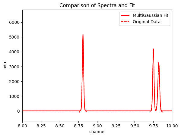
Ir_multi = MultiBatchGaussian(Ir_img, xs = wavelengths, num_peaks = 15)

Ir_multi.fit()

f, ax = plt.subplots()
Ir_multi.plot_fit(ax = ax)
ax.set_xlim([8, 10])

centroids = Ir_multi.get_centroids_ascending()
print(centroids)

[[8.80910866e+00 1.68642086e-04]
 [9.75019873e+00 2.72684748e-04]
 [9.82194180e+00 4.04853965e-04]
 [1.06157482e+01 2.49820935e-04]
 [1.11146555e+01 3.14898435e-04]
 [1.16694731e+01 2.06514901e-04]
 [1.22649749e+01 7.09158037e-04]
 [1.27676838e+01 3.55130947e-04]
 [1.30307583e+01 1.15214130e-03]
 [1.42644909e+01 1.05170271e-03]
 [1.43306900e+01 1.94775210e-04]
 [1.47131903e+01 1.07046281e-03]
 [1.72600294e+01 6.53520247e-04]
 [1.76197812e+01 3.37757159e-04]
 [1.95091402e+01 4.71991992e-04]]

Note that because we gave the wavelengths as the x-values when we created the MultiBatchGaussian, centroids (and their centroid uncertainties) are already in nm. The next step is to calculate the total uncertainty for each centroid. The total uncertainty has three parts

\(u_{x,nm}\), the centroid uncertainty
\(u_{cal}\), the calibration uncertainty
\(u_{sys}\), the systematic uncertainty.

To calculate the total uncertainty, combine all parts in quadrature:

\[u_{tot} = \sqrt{{u_x,nm} ^ 2 + {u_cal} ^ 2 + {u_sys} ^ 2}\]

\(u_{sys}\) is easily gotten through the cal.systematic_uncertainty

sys_unc = Ne_cal.systematic_uncertainty

The calibration uncertainty can be found by linearly interpolating the confidence band array. For example, if the calibration uncertainty at channel 1000 is 0.001 nm, but is 0.0012 nm at channel 1001, then a peak with a center at channel 1000.5 would have calibration uncertainty 0.0011 nm. Note that the calibration uncertainty generally changes slowly.

#the calibration uncertainty changes with wavelength, so we need to calculate it
#for each centroid


calibration_unc = [np.interp(centroid, wavelengths, Ne_cal.confidence_bands(n_sigma = 1)) \
            for centroid in centroids[:, 0]]

Finally, we can calculate the total uncertainty for each centroid using the formula above:

for centroid, centroid_uncertainty, cal_unc in zip(centroids[:, 0], centroids[:, 1], calibration_unc):
    total_unc = np.sqrt(centroid_uncertainty ** 2 + cal_unc ** 2 + sys_unc ** 2)

    print(f'{centroid:4.4f} +/- {total_unc:5.4f}')

8091 +/- 0.0013
7502 +/- 0.0012
8219 +/- 0.0013
6157 +/- 0.0012
1147 +/- 0.0012
6695 +/- 0.0012
2650 +/- 0.0013
7677 +/- 0.0012
0308 +/- 0.0016
2645 +/- 0.0016
3307 +/- 0.0012
7132 +/- 0.0016
2600 +/- 0.0014
6198 +/- 0.0014
5091 +/- 0.0023

These are the values that should be published in a paper. They take into account not only the fit uncertainty, but also the calibration and systematic uncertainties.

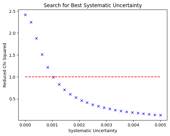
Estimation of Systematic Uncertainty#

One measure of goodness-of-fit is the reduced chi-squared (A.K.A. \(\chi^2_{\nu}\)), defined as:

\[\chi^2_{\nu} = \frac{1}{n - m} \sum{\frac{(y_{observed} - y_{calculated})^2}{\sigma ^ 2}}\]

If there are no systematic errors in your experiment, then \(\chi^2_{\nu}\) should be close to 1. Values significantly less than 1 suggest you are overestimating your uncertainties, while values greater than 1 suggest you are underestimating your uncertainties.

To reduce the chance of publishing over confident uncertainties, euv_fitting adds a systematic uncertainty in quadrature with the channel and literature uncertainties if the \(\chi^2_{\nu}\) is greather than 1. The systematic uncertainty is slowly increased until \(\chi^2_{\nu}\) equals 1, as shown below.